UNDERSTANDING PROPENSITY SCORES
From naïve enthusiasm to intuitive understanding [1]

New methodologies have been emerging to estimate the effect of a binary exposure on an outcome or result. Propensity scores has been proven to be useful to estimate the causal effect of exposure under certain assumptions even in the presence of confounding variables. This paper aims to define what is causal effect, detail how the propensity score can estimate causal effects as well as the assumptions and concerns about this method using an example of exposure to breast milk and the infant’s consequent neurodevelopment (IQ) after 7.5 years. In this example, each individual has two potential outcomes, one in the individual was exposed to breastfeeding or not but only one outcome can be observed from the data and the other outcome is defined as counterfactual. Therefore, the causal effect can be defined as the mean of the individual causal effect and can be estimated by using results of other individuals to calculate counterfactual outcomes that were not observed.
Three different causal effects are of interest and are used depending on the questions that wants to be answered: the Average Causal Effect of the Exposure (ACEALL) which is the causal effect in the entire population, the Average Causal Effect of the Exposure on the Exposed (ACEEXP) which considers the subgroup of the population that is exposed, and the Average Causal Effect of the Unexposed (ACEUNE) that considers the subgroup of the unexposed.
Given that is our intention to convert causal estimands to statistical estimands as part of the identification step, a few assumptions and properties are needed. For this specific example taken from [1] the intention is to be able to estimate the Average Treatment Effect represented by E[Y_1-Y_0] using propensity scores. The assumptions made were that the treatment assignment precedes the effect Y, that every subject must have the potential to be exposed and unexposed, Stable Unit Treatment Value Assumption (SUTVA) given that data were sample independently from the population and that there are not unobserved confounders. This last assumption is also known as Strongly Ignorable Treatment Assignment (SITA) given that the observed covariates are conditionally independent.
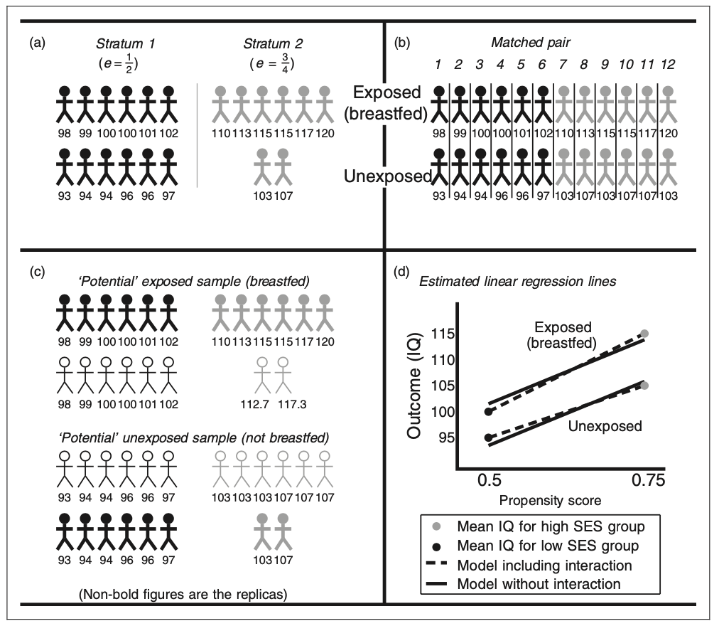
Causal Effects can be estimated using four different propensity scores methods: stratification, matching, inverse weighting, and covariate adjustment. The stratification method consists of making strata or groups of the individuals who have the same propensity score, estimating the exposure effect between exposed and unexposed group and using a weighted average. The matching method consist of pairing each exposed individual with another unexposed with the same propensity score and calculating the average pair estimate of the effect of the exposure after taking the difference in the two outcomes of within-pair effect. The inverse weighting creates two potential samples, each one for each outcome, assigning a replica to the original individual’s outcome based on the propensity score and individual’s characteristics. That is, if the propensity score is 1/2 for low-income individuals, then the replica should have the same number of individuals for high income entities and the same outcome of the original individual. Finally, the covariate adjustment can be estimated using a linear regression where the dependent variable would be the outcome and the independent variables to be the exposure and the propensity score. The regression coefficient for the propensity score variable should result in the estimate of the exposure effect. Figure 2 provides a graphical representation of the four different estimation methods.
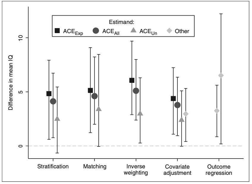
Choosing a method and estimating the propensity score is not considered to be a trivial decision given that each one has advantages and disadvantages. Propensity scores are often estimated using logistic regression using all the confounders, but other non and semi-parametric approaches to this model have been proposed. In the breastfeeding example, a total of 926 babies were considered and were assessed at approximately 7.5 years of age by measuring their IQ. Additionally, other variables like social class, mother’s education, family structure, marital status, infant age and gender, birthweight and birth order were considered. Propensity scores were estimated using a logistic regression and the three causal effects were calculated with the four methods but only 487 follow-up samples were collected. Results show that each methods performance was similar as shown in Figure 3, suggesting a positive relationship between breast milk consumption and IQ.
Causal inference is still a topic that deserves to be investigated more rigorously. Although relevance has been found in the studies carried out, there is still debate about the assumptions that are needed for these models to be used. Many of the areas of interest include estimating confidence intervals for propensity scores, using these propensity scores to train nonparametric models, and establishing a consensus for their proper use.
A Working Example
Definition
The intention of this project is to provide a detailed explanation of the procedure of estimating average treatment effects using propensity scores and matching. For this, the NHEFS data set from 1629 cigarette smokers aged 25-74 years who had a baseline visit and a follow-up visit about 10 years later.
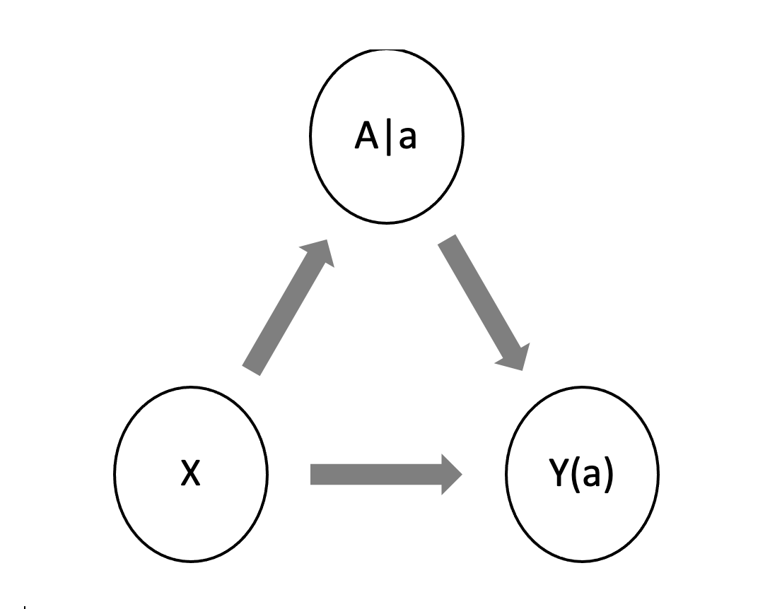
Figure 4 shows the appropriate Single World Intervention Graph (SWIG) for this problem that is used to represent potential outcomes and their conditional independence relations where X are the covariates of the, A is the treatment and Y is the outcome.
Identification
In this example, the following steps demonstrates how to estimate the Average Treatment Effect $ ATE_{all} $
Assumptions:
- $ Y\left(a\right)\bot A|e(x) $
- Consistency
First, we are going to look at
In second place, if Y\left(a\right)\bot A|e(x) and because of consistency:
Then, Because of the Law of iterated Expectations:
Therefore,
In the last equation, we showed that it is possible to estimate the Average Treatment Effect from the data provided.
Estimation & Sensitivity Analysis
Propensity Scores
Bryan S. Ortiz-Torres
11/15/2022
A Working Example
To show that the procedure to estimate the causal effect using propensity scores, a logistic regression was performed to determine the propensity scores and the matching procedure was followed to estimate the average treatment effect using the NHEFS data from 1629 cigarette smokers aged 25-74 years who had a baseline visit and a follow-up visit about 10 years later.
library(knitr)
opts_chunk$set(warning = FALSE, message = FALSE)
library(sandwich)
library(cobalt)
#library(kableExtra)
library(tidyverse)
library(broom)
library(estimatr)
library(fastDummies)
library(glmnet)
library(dplyr)
library(marginaleffects)
library(twang)
library(WeightIt)
library(gdata)
library(stats)
I. Data and Parameters
library(readxl)
Project_Data <- data.frame(read_excel("/Users/bryanortiz/OneDrive - UW-Madison/Causal Inference/Project/Project_Data_Hernan.csv"))
columns <- c("active","age","alcoholfreq","asthma","birthplace","bronch", "cholesterol","diabetes","education","hepatitis","hf","race", "sex", "tumor","weakheart","qsmk","wt82_71")


df <- Project_Data[,columns]
df=df[complete.cases(df),]

#c(qsmk,active,age,alcoholfreq,asthma,birthplace,bronch,cholesterol,diabetes, education, hepatitis, hf, race, sex, tumor, weakheart)]
II. Calculating Propensity Scores using Logistic Regression
The first step to implement this methodology is to estimate the propensity scores. In this case, a logistic regression was performed where the response variable is “quit smoking”. After that, propensity scores were obtained by extracting the response of the logistic regression model.
propensity_model <- glm(qsmk ~(active + age+ alcoholfreq + asthma + birthplace + bronch + cholesterol+ diabetes + education + hepatitis + hf + race + sex + tumor + weakheart), family="binomial",data = df)

# calculate predicted propensity scores
df$ps_lgt <- predict(propensity_model, type = "link") #logit
df$ps <- predict(propensity_model, type = "response")
# Create contingency table
df = df%>%
mutate(
Change = ifelse(wt82_71 >= 0,"Increase","Decrease"),
quitsmoking = factor(qsmk,levels = 0:1, labels = c("No","Yes"))
)
results <- table(df$quitsmoking,df$Change)
results##
## Decrease Increase
## No 382 702
## Yes 95 281The graph shows the distribution of estimated propensity score logits among individuals who do not quit smoking and individuals who quit smoking It can be seen that some extrapolation is present.
library(base)
ps_density <-
  ggplot(df, aes(ps_lgt, group = quitsmoking,fill = as.factor(quitsmoking))) +
  geom_density(alpha = 0.3, trim = TRUE) +
  scale_fill_brewer(type = "qual", palette = 6) +
  theme_minimal() +
  theme(legend.position = c(0.9, 0.9)) +
  labs(fill = "", x = "Logit propensity score")
ps_density
Summary of Propensity Scores Results
group_by(df, qsmk) %>% summarize(min = min(ps_lgt), mean = mean (ps_lgt), max = max(ps_lgt))Matching
In this section, different matching techniques were performed to estimate the average treatment effect.
Nearest Neighbor
library(MatchIt)

NN_match <- matchit(qsmk ~(active + age+ alcoholfreq + asthma + birthplace + bronch + cholesterol+ diabetes + education + hepatitis + hf + race + sex + tumor + weakheart),data = df,distance = "logit", method = "nearest")
summary(NN_match)$nn
## Control Treated
## All (ESS) 1084 376
## All 1084 376
## Matched (ESS) 376 376
## Matched 376 376
## Unmatched 708 0
## Discarded 0 03-1 matching with replacement:
NNreplace_match <- matchit(qsmk ~(active + age+ alcoholfreq + asthma + birthplace + bronch + cholesterol+ diabetes + education + hepatitis + hf + race + sex + tumor + weakheart),data = df,
                    distance = "logit",
                    method = "nearest",
                    replace= TRUE,
                    ratio = 3
                    )
summary(NNreplace_match)$nn
## Control Treated
## All (ESS) 1084.000 376
## All 1084.000 376
## Matched (ESS) 450.242 376
## Matched 628.000 376
## Unmatched 456.000 0
## Discarded 0.000 0Balance Method Comparison:
dropstatus_wts <- data.frame(
  NN = get.w(NN_match),
  NNreplace = get.w(NNreplace_match)
)
# Balance table
(NN_NNreplace_balance <-
  bal.tab(qsmk ~(active + age+ alcoholfreq + asthma + birthplace + bronch + cholesterol+ diabetes + education + hepatitis + hf + race + sex + tumor + weakheart),data = df,
                    weights = dropstatus_wts,
                    un = TRUE))
## Balance Measures
## Type Diff.Un Diff.NN Diff.NNreplace
## active Contin. 0.0956 0.0643 0.0589
## age Contin. 0.2543 0.0098 -0.0124
## alcoholfreq Contin. 0.0471 -0.0369 -0.0266
## asthma Binary 0.0213 -0.0106 0.0018
## birthplace Contin. -0.0800 0.0165 -0.0087
## bronch Binary 0.0047 0.0053 0.0018
## cholesterol Contin. 0.0941 -0.0191 -0.0126
## diabetes Contin. -0.0513 -0.0240 0.0027
## education Contin. 0.1148 0.0021 0.0070
## hepatitis Binary -0.0025 -0.0080 -0.0062
## hf Binary -0.0002 0.0053 0.0018
## race Binary -0.0680 0.0027 -0.0053
## sex Binary -0.0704 -0.0346 0.0080
## tumor Binary -0.0019 0.0027 0.0044
## weakheart Binary -0.0036 0.0133 0.0044
##
## Effective sample sizes
## Control Treated
## All 1084. 376
## NN 376. 376
## NNreplace 450.24 376Love Plot Comparison:
love.plot(NN_NNreplace_balance,
          threshold = 0.1,
          colors = c("red","blue","purple"),
          size = 3, alpha = 0.7) +
  theme_minimal()
Final balance assessment for 3-1 matching with replacement:
bal.tab(NNreplace_match, un = TRUE)## Balance Measures
## Type Diff.Un Diff.Adj
## distance Distance 0.4345 0.0009
## active Contin. 0.0956 0.0589
## age Contin. 0.2543 -0.0124
## alcoholfreq Contin. 0.0471 -0.0266
## asthma Binary 0.0213 0.0018
## birthplace Contin. -0.0800 -0.0087
## bronch Binary 0.0047 0.0018
## cholesterol Contin. 0.0941 -0.0126
## diabetes Contin. -0.0513 0.0027
## education Contin. 0.1148 0.0070
## hepatitis Binary -0.0025 -0.0062
## hf Binary -0.0002 0.0018
## race Binary -0.0680 -0.0053
## sex Binary -0.0704 0.0080
## tumor Binary -0.0019 0.0044
## weakheart Binary -0.0036 0.0044
##
## Sample sizes
## Control Treated
## All 1084. 376
## Matched (ESS) 450.24 376
## Matched (Unweighted) 628. 376
## Unmatched 456. 0Matching: treatment effect estimation
Estimation of the ATE based on the mean differences in the outcome between treated and untreated units in the (new and improved) matched sample.
NNreplace_match_dat <- match.data(NNreplace_match)
NNreplace_match_dat <- data.frame(NNreplace_match_dat)

NNreplace_meandiff <- lm_robust(wt82_71 ~ qsmk, weights = weights, data = NNreplace_match_dat)
summary(NNreplace_meandiff)
##
## Call:
## lm_robust(formula = wt82_71 ~ qsmk, data = NNreplace_match_dat,
## weights = weights)
##
## Weighted, Standard error type: HC2
##
## Coefficients:
## Estimate Std. Error t value Pr(>|t|) CI Lower CI Upper DF
## (Intercept) 1.463 0.3460 4.229 2.560e-05 0.7843 2.142 1002
## qsmk 3.195 0.5675 5.630 2.338e-08 2.0816 4.309 1002
##
## Multiple R-squared: 0.03628 , Adjusted R-squared: 0.03532
## F-statistic: 31.7 on 1 and 1002 DF, p-value: 2.338e-08Estimation of the ATE using ANCOVA within the (new and improved) matched sample.
NNreplace_ancova <- lm_robust(wt82_71 ~ (qsmk + active + age+ alcoholfreq + asthma + birthplace + bronch + cholesterol+ diabetes + education + hepatitis + hf + race + sex + tumor + weakheart), weights = weights, data = NNreplace_match_dat)
summary(NNreplace_ancova)
##
## Call:
## lm_robust(formula = wt82_71 ~ (qsmk + active + age + alcoholfreq +
## asthma + birthplace + bronch + cholesterol + diabetes + education +
## hepatitis + hf + race + sex + tumor + weakheart), data = NNreplace_match_dat,
## weights = weights)
##
## Weighted, Standard error type: HC2
##
## Coefficients:
## Estimate Std. Error t value Pr(>|t|) CI Lower CI Upper DF
## (Intercept) 9.334869 1.853778 5.0356 5.661e-07 5.697069 12.972669 987
## qsmk 3.229084 0.548296 5.8893 5.313e-09 2.153125 4.305043 987
## active -1.148901 0.426931 -2.6911 7.243e-03 -1.986697 -0.311104 987
## age -0.152635 0.024637 -6.1953 8.529e-10 -0.200982 -0.104287 987
## alcoholfreq 0.142770 0.214513 0.6656 5.059e-01 -0.278184 0.563723 987
## asthma -0.184216 1.397777 -0.1318 8.952e-01 -2.927173 2.558742 987
## birthplace 0.038967 0.019693 1.9787 4.813e-02 0.000322 0.077611 987
## bronch 0.103258 0.960372 0.1075 9.144e-01 -1.781349 1.987864 987
## cholesterol -0.006804 0.006202 -1.0972 2.728e-01 -0.018974 0.005366 987
## diabetes 0.155842 0.278342 0.5599 5.757e-01 -0.390369 0.702053 987
## education 0.108910 0.228913 0.4758 6.343e-01 -0.340302 0.558121 987
## hepatitis 0.456220 1.322645 0.3449 7.302e-01 -2.139299 3.051738 987
## hf 3.533200 5.147966 0.6863 4.927e-01 -6.569016 13.635416 987
## race -1.728514 0.982938 -1.7585 7.897e-02 -3.657403 0.200374 987
## sex -0.732232 0.547984 -1.3362 1.818e-01 -1.807578 0.343115 987
## tumor -1.654336 1.587272 -1.0423 2.976e-01 -4.769152 1.460480 987
## weakheart -1.538751 2.766813 -0.5561 5.782e-01 -6.968262 3.890760 987
##
## Multiple R-squared: 0.1238 , Adjusted R-squared: 0.1096
## F-statistic: 7.007 on 16 and 987 DF, p-value: 1.716e-15Estimation of the ATT using regression (possibly with weights) within the matched sample.
NNreplace_reg <- lm_robust(wt82_71 ~ (qsmk + active + age+ alcoholfreq + asthma + birthplace + bronch + cholesterol+ diabetes + education + hepatitis + hf + race + sex + tumor + weakheart), weights = weights, data = NNreplace_match_dat)

#ATT
ATTmatch <- marginaleffects(NNreplace_reg, variables = "qsmk")
summary(ATTmatch)
II. Sensitivity Analysis
Sensitivity Analsys can be done to determine potential impact using other estimation models, matching methods and the violation of the unobserved confounding assumption. For the estimation of the average treatment effec the assumptions previously made were \(Y\left(a\right)\bot A|e(x)\) , Consistency and no unmeasured confounders. For the later, the Rosenbound sensitivity analysis for binary outcomes was performed to illustrate how big the parameter Gamma must be so that the Risk Ratio of the unmeasured confounder given the treatment is bigger than the Risk Ratio of the outcome given the treatment. Additionally, it is assumed that this ratios are greater than 1.
# Using the Rosenbaum  approach for binary variables
library(rbounds)
sensitivity=as.matrix.data.frame(binarysens(x=702,y=95, Gamma = 10, GammaInc = 0.2)$bounds)
kable(sensitivity[20:46,])| Gamma | Lower bound | Upper bound |
|---|---|---|
| 4.8 | 0 | 0.00001 |
| 5.0 | 0 | 0.00007 |
| 5.2 | 0 | 0.00034 |
| 5.4 | 0 | 0.00124 |
| 5.6 | 0 | 0.00382 |
| 5.8 | 0 | 0.01003 |
| 6.0 | 0 | 0.02291 |
| 6.2 | 0 | 0.04626 |
| 6.4 | 0 | 0.08380 |
| 6.6 | 0 | 0.13804 |
| 6.8 | 0 | 0.20918 |
| 7.0 | 0 | 0.29478 |
| 7.2 | 0 | 0.39006 |
| 7.4 | 0 | 0.48892 |
| 7.6 | 0 | 0.58521 |
| 7.8 | 0 | 0.67378 |
| 8.0 | 0 | 0.75113 |
| 8.2 | 0 | 0.81559 |
| 8.4 | 0 | 0.86708 |
| 8.6 | 0 | 0.90665 |
| 8.8 | 0 | 0.93601 |
| 9.0 | 0 | 0.95711 |
| 9.2 | 0 | 0.97185 |
| 9.4 | 0 | 0.98188 |
| 9.6 | 0 | 0.98854 |
| 9.8 | 0 | 0.99287 |
| 10.0 | 0 | 0.99563 |
HTML Document
Conclusion
In summary, the intention of this project was to show how to estimate causal effects using propensity scores as shown in the paper Propensity scores: From naïve enthusiasm to intuitive understanding using the NHFES data set that includes. In this case, the intention was to estimate the effect on smoking to gaining weight given a set of covariates. Our major finding was that using propensity scores and different matching techniques, the estimation of the average treatment effect was 3.29 when using the nearest neighbor algorithm and a 3 to 1 ratio to match treated individuals to non-treated individuals. Possible avenues for future work include using different matching methods like an optimal matching using propensity scores or making an optimal matching by including the balancing function in the objective function and compare both results.
References
- Williamson, E., Morley, R., Lucas, A., & Carpenter, J. (2011). Propensity scores: From naïve enthusiasm to intuitive understanding. Statistical Methods in Medical Research, 21(3), 273–293. https://doi.org/10.1177/0962280210394483
- Rosenbaum PR and Rubin DB. The central role of the propensity score in observational studies for causal effects. Biometrika 1983; 70: 41–55.
- Senn S, Graf E and Caputo A. Stratification for the propensity score compared with linear regression techniques to assess the effect of treatment or exposure. Stat Med 2007; 26: 5529–5544.
- D’Agostino RB. Propensity score methods for bias reduction in the comparison of a treatment to a non- randomized control group. Stat Med 1998; 17: 2265–2281.
- Joffe MM and Rosenbaum PR. Invited commentary: Propensity scores. Am J Epidemiol 1999; 150: 327–333.
- Austin PC and Mamdani MM. A comparison of propensity score methods: A case-study estimating the effectiveness of post-AMI statin use. Stat Med 2006; 25: 2084–2106.
- Kurth T, Walker AM, Glynn RJ, et al. Results of multivariable logistic regression, propensity matching, propensity adjustment, and propensity-based weighting under conditions of nonuniform effect. Am J Epidemiol 2006; 163: 262–270.
- Weschler D. Weschler Intelligence Scale for Children, Anglicized revised edition. Sidcup, Kent: The Psychological Corporation Ltd.; 1974.
- Paul R. Rosenbaum, Donald B. Rubin, The central role of the propensity score in observational studies for causal effects, Biometrika, Volume 70, Issue 1, April 1983, Pages 41–55,